Importing Data Into R from Different Sources

I have found that I get data from many different sources.  These sources range from simple .csv files to more complex relational databases, to structure XML or JSON files.  I have compiled the different approaches that one can use to easily access these datasets.

Local Column Delimited Files

This is probably the most common and easiest approach to load data into R.  It simply requires one line to do everything that is needed to set up the data.  Then a couple additional lines to tidy up the dataset.

file <- "c:\\my_folder\\my_file.txt" raw_data <- read.csv(file, sep=",");  ##'sep' can be a number of options including \t for tab delimited names(raw_data) <- c("VAR1","VAR2","RESPONSE1") [/sourcecode] Text File From the Internet

I find this very useful when I need to get datasets from a Web site.  This is particularly useful if I need to rerun the script and the Web site continually updates their data.  This save me from having to download the dataset into a csv file each time I need to run an update.  In this example I use one of my favorite data sources which comes from the National Data Buoy Center.  This example pulls data from a buoy (buoy #44025) off the coast of New Jersey.  Conveniently you can use the same read.csv() function that you would use if read the file from you own computer.  You simply replace the file location with the URL of the data.

file <- "http://www.ndbc.noaa.gov/view_text_file.php?filename=44025h2011.txt.gz&dir=data/historical/stdmet/

raw_data <- read.csv(file, header=T, skip=1) [/sourcecode] Files From Other Software

Often I will have Excel files, SPSS files, or SAS dataset set to me.  Once again I can either export the data as a csv file and then import using the read.csv function.  However, taking that approach every time means that there is an additional step.  By adding unnecessary steps to a process increases the risk that the data might get corrupted due to human error.  Furthermore, if the data is updated from time to time then the data that you downloaded last week may not have the most current data.


SPSS

library(foreign)
file <- "C:\\my_folder\\my_file.sav" raw <- as.data.frame(read.spss(file)) [/sourcecode]   Microsoft Excel

library(XLConnect)

file <- "C:\\my_folder\\my_file.xlsx" raw_wb <- loadWorkbook(file, create=F) raw <- as.data.frame( readWorksheet(raw_wb, sheet='Sheet1') ) [/sourcecode] Data From Relational Databases

There is the RMySQL library which is very useful.  However, I have generally been in the habit of using the RODBC library.  The reason for this is that I will often jump between databases (e.g. Oracle, MSSQL, MySQL).  By using the RODBC library I can keep all of my connections in one location and use the same functions regardless of the databases.  This example below will work on any standard SQL database.  You just need to make sure you set up an ODBC connection call (in this example) MY_DATABASE.

library(RODBC)
channel <- odbcConnect("MY_DATABASE", uid="username", pwd="password") raw <- sqlQuery(channel, "SELECT * FROM Table1"); [/sourcecode] Data from Non-Relational Databases

R has the capability to pull data from non-relational databases.  These include Hadoop (rhbase), Cassandra (RCassandra), MongoDB (rmongodb).  I personally have not used RCassandra but here is the documentation.  The example here uses MongoDB using an example provided by MongoDB.

library(rmongodb)
MyMongodb <- "test" ns <- "articles" mongo <- mongo.create(db=MyMmongodb) list.d <- mongo.bson.from.list(list( "_id"="wes", name=list(first="Wesley", last=""), sex="M", age=40, value=c("7", "5","8","2") )) mongo.insert(mongo, "test.MyPeople", list.d) list.d2 <- mongo.bson.from.list(list( "_id"="Article1", when=mongo.timestamp.create(strptime("2012-10-01 01:30:00", "%Y-%m-%d %H:%M:%s"), increment=1), author="wes", title="Importing Data Into R from Different Sources", text="Provides R code on how to import data into R from different sources.", tags=c("R", "MongoDB", "Cassandra","MySQL","Excel","SPSS"), comments=list( list( who="wes", when=mongo.timestamp.create(strptime("2012-10-01 01:35:00", "%Y-%m-%d %H:%M:%s"), increment=1), comment="I'm open to comments or suggestions on other data sources to include." ) ) ) ) list.d2 mongo.insert(mongo, "test.MyArticles", list.d2) res <- mongo.find(mongo, "test.MyArticles", query=list(author="wes"), fields=list(title=1L)) out <- NULL while (mongo.cursor.next(res)){ out <- c(out, list(mongo.bson.to.list(mongo.cursor.value(res)))) } out [/sourcecode]   Copied and Pasted Text

raw_txt <- " STATE READY TOTAL AL 36 36 AK 5 8 AZ 15 16 AR 21 27 CA 43 43 CT 56 68 DE 22 22 DC 7 7 FL 130 132 GA 53 54 HI 11 16 ID 11 11 IL 24 24 IN 65 77 IA 125 130 KS 22 26 KY 34 34 LA 27 34 ME 94 96 MD 25 26 MA 82 92 Mi 119 126 MN 69 80 MS 43 43 MO 74 82 MT 34 40 NE 9 13 NV 64 64 NM 120 137 NY 60 62 NJ 29 33 NH 44 45 ND 116 135 NC 29 33 OH 114 130 OK 19 22 PA 101 131 RI 32 32 Sc 35 45 SD 25 25 TN 30 34 TX 14 25 UT 11 11 VT 33 49 VA 108 124 WV 27 36 WI 122 125 WY 12 14 " raw_data <- textConnection(raw_txt) raw <- read.table(raw_data, header=TRUE, comment.char="#", sep="") close.connection(raw_data) raw ###Or the following line can be used raw <- read.table(header=TRUE, text=raw_txt) [/sourcecode]  Structured Local or Remote Data

One feature that I find quite useful is when there is a Web site with a table that I want to analyze.  R has the capability to read through the HTML and import the table that you want.  This example uses the XML library and pulls down the population by country in the world.  Once the data is brought into R it may need to be cleaned up a bit removing unnecessary columns and other stray characters.  The examples here use remote data from other Web sites.  If the data is available as a local file then it can be imported in a similar fashion just using filename rather than the URL.

library(XML)

url <- "http://en.wikipedia.org/wiki/List_of_countries_by_population" population = readHTMLTable(url, which=3) population [/sourcecode] Or you can use the feature to simple grab XML content.  I have found this particularly useful when I need geospatial data and need to get the latitude/longitude of a location (this example uses Open Street Maps API provided by MapQuest).  This example obtains the results for the coordinates of the United States White House. [sourcecode language="css"] url <- "http://open.mapquestapi.com/geocoding/v1/address?location=1600%20Pennsylvania%20Ave,%20Washington,%20DC&outFormat=xml" mygeo <- xmlToDataFrame(url) mygeo$result [/sourcecode] An alternate approach is to use a JSON format.  I generally find that JSON is a better format and it can be readily used in most programming languages. [sourcecode language="css"] library(rjson) url <- "http://open.mapquestapi.com/geocoding/v1/address?location=1600%20Pennsylvania%20Ave,%20Washington,%20DC&outFormat=json" raw_json <- scan(url, "", sep="\n") mygeo <- fromJSON(raw_json) [/sourcecode]

Plotting Likert Scales

Graphs can provide an excellent way to emphasize a point and to quickly and efficiently show important information. Sadly, poor graphs can be a good way to waste space in an article, take up time in a presentation, and waste a lot of ink all while providing little to no information.

Excel has made it possible to make all sort of graphs. However, just because the graph looks like a spider web or like something you can eat for dessert doesn’t mean you should use it.

This discussion here will show five options on how to graph Likert scale data, will show best/common practice for graphing, and will provide the R code for each graph. These graphing approaches are based on a list that I have compiled that the different people that I have worked with have used to graph and interpret Likert scales within their organization.

Likert scales usually have 5 or 7 response options. However, the exact number and whether there should be an odd or even number of responses is a topic for another psycometric discussion. A typical Likert scale is:

1 Strongly Agree
2 Agree
3 Neutral
4 Disagree
5 Strongly Disagree

For example purposes I generated some random discrete data that is formatted as a Likert scale.   I have created three examples to show the extremities of Likert scale responses.


set.seed(1234)
library(e1071)
probs <- cbind(c(.4,.2/3,.2/3,.2/3,.4),c(.1/4,.1/4,.9,.1/4,.1/4),c(.2,.2,.2,.2,.2))
my.n <- 100
my.len <- ncol(probs)*my.n
raw <- matrix(NA,nrow=my.len,ncol=2)
raw <- NULL
for(i in 1:ncol(probs)){
raw <- rbind(raw, cbind(i,rdiscrete(my.n,probs=probs&#91;,i&#93;,values=1:5)))
}

r <- data.frame( cbind(
as.numeric( row.names( tapply(raw&#91;,2&#93;, raw&#91;,1&#93;, mean) ) ),
tapply(raw&#91;,2&#93;, raw&#91;,1&#93;, mean),
tapply(raw&#91;,2&#93;, raw&#91;,1&#93;, mean) + sqrt( tapply(raw&#91;,2&#93;, raw&#91;,1&#93;, var)/tapply(raw&#91;,2&#93;, raw&#91;,1&#93;, length) ) * qnorm(1-.05/2,0,1),
tapply(raw&#91;,2&#93;, raw&#91;,1&#93;, mean) - sqrt( tapply(raw&#91;,2&#93;, raw&#91;,1&#93;, var)/tapply(raw&#91;,2&#93;, raw&#91;,1&#93;, length) ) * qnorm(1-.05/2,0,1)
))
names(r) <- c("group","mean","ll","ul")

gbar <- tapply(raw&#91;,2&#93;, list(raw&#91;,2&#93;, raw&#91;,1&#93;), length)

sgbar <- data.frame( cbind(c(1:max(unique(raw&#91;,1&#93;))),t(gbar)) )

sgbar.likert<- sgbar&#91;,2:6&#93;

&#91;/sourcecode&#93;

<strong>Diverging Stacked Bar Chart</strong>

Diverging stacked bar charts are often the best choice when visualizing Likert scale data.  There are various ways to produce these graphs but I have found the easiest approach uses the <em>HH </em>package.  There are many graphs that can be produced using this package. I have provided three approaches here.


require(grid)
require(lattice)
require(latticeExtra)
require(HH)
sgbar.likert<- sgbar&#91;,2:6&#93;
likert(sgbar.likert,
main='Example Diverging Stacked Bar Chart for Likert Scale',
sub="Likert Scale")

likert(sgbar.likert, horizontal=FALSE,
aspect=1.5,
main="Example Diverging Stacked Bar Chart for Likert Scale",
auto.key=list(space="right", columns=1,
reverse=TRUE, padding.text=2),
sub="Likert Scale")

likert(sgbar.likert,
auto.key=list(between=1, between.columns=2),
xlab="Percentage",
main="Example Diverging Stacked Bar Chart for Likert Scale",
BrewerPaletteName="Blues",
sub="Likert Scale")

&#91;/sourcecode&#93;
<p style="text-align: center;"><a href="http://statistical-research.com/wp-content/uploads/2012/12/divergingstacked_h.likert.png"><img class="aligncenter  wp-image-859" title="Diverging Stacked Bar Chart for Likert Scale" src="http://statistical-research.com/wp-content/uploads/2012/12/divergingstacked_h.likert.png" alt="" width="452" height="256" /></a></p>
<p style="text-align: center;"><a href="http://statistical-research.com/wp-content/uploads/2012/12/divergingstacked_v.likert.png"><img class="aligncenter  wp-image-860" title="Diverging Stacked Bar Chart (Vertical) for Likert Scale" src="http://statistical-research.com/wp-content/uploads/2012/12/divergingstacked_v.likert.png" alt="" width="502" height="284" /></a></p>
<p style="text-align: center;"><a href="http://statistical-research.com/wp-content/uploads/2012/12/divergingstacked_h_blue.likert.png"><img class="aligncenter  wp-image-861" title="Diverging Stacked Bar Chart for Likert Scale Using Blue Tones" src="http://statistical-research.com/wp-content/uploads/2012/12/divergingstacked_h_blue.likert.png" alt="" width="452" height="256" /></a></p>
<strong>Mean Value</strong>

Often researchers will simply take each response option and interpret it as a real number.  Using this approach makes it very convenient to calculate the mean value and standard deviation (and confidence intervals). This is particularly useful when working with non-analytical clients.  However, this is a controversial issue. Taking this approach requires a lot of statistical assumptions that may not be correct. For starters the response options really need to be equidistant from each other. For example, is the distance from <em>Strongly Agree</em> to <em>Agree</em> the same distance from <em>Disagree</em> to <em>Strongly Disagree</em>? This may be true for one question but it might not be true for all questions on a questionnaire. Different questions and question wording are quite likely going to have different distributions. Furthermore, confidence intervals require normality assumptions which may also be incorrect.

What makes matters worse is that if there are 50 respondents and 25 of them mark <em>Strongly Disagree</em> and 25 of them mark <em>Strongly Agree</em> then the mean will be 3 implying that, on average, the results are neutral.  But that clearly does not adequately describe the data. Ultimately, it is up to the statistician to work with the client to use an appropriate method that appropriately conveys the message and that both parties can agree upon.


plot.new(); par(mfrow=c(1,1));

plot(r$group,r$mean, type="o", cex=1, col="blue", pch=16,
ylim=c(1,5), lwd=2,
, ylab="Mean Value", xlab="Group"
, main=paste("Likert Scale Mean Values Example")
, cex.sub=.60
, xaxt = "n", yaxt = "n");
axis(1, at=(1:3), tcl = -0.7, lty = 1, lwd = 0.8, labels=TRUE)
axis(2, at=(1:5), labels=TRUE, tcl = -0.7, lty = 1)
abline(h=c(1:5), col="grey")
lines(r$group,r$ll, col='red', lwd=2)
lines(r$group,r$ul, col='red', lwd=2)

legend("topright", c("Mean","Confidence Interval"),
col=c('blue','red'), title="Legend",
lty=1, lwd=2,
inset = .05)

Pies and Multiple Pies

A table is nearly always better than a dumb pie chart; the only worse design than a pie chart is several of them, for then the viewer is asked to compare quantities located in spatial disarray both within and between charts (…). Given their low density and failure to order numbers along a visual dimension, pie charts should never be used. — Edward Tufte

Pie charts are notoriously difficult to convey the information that was intended.  As far as pie charts go I don’t ever use them.  There are far better ways to visualize data.  However, I have heard some people give a reason for using them that are somewhat justified and generally are based on the ‘eye candy’ argument.  But as far as creating a graph that both provides information and looks good a 3-D pie chart is probably not the best choice.  I debated whether I should even include the R code for the example but to provide full disclosure here’s the code.


my.table <- table(raw&#91;,2&#93;&#91;raw&#91;,1&#93;==1&#93;)

names(my.table) <- c("Strongly Agree","Agree","Neutral","Disagree","Strongly Disagree")
labl <- paste(names(my.table), "\n", my.table, sep="")
pie(my.table, labels=labl, main="Example Pie Chart of Likert Scale")

&#91;/sourcecode&#93;
<p style="text-align: center;"><a href="http://statistical-research.com/wp-content/uploads/2012/12/pie.likert.png"><img class="aligncenter  wp-image-852" title="Pie Chart for Likert Scale" src="http://statistical-research.com/wp-content/uploads/2012/12/pie.likert.png" alt="" width="420" height="262" /></a></p>


plot.new()
num.groups <- length(unique(raw&#91;,1&#93;))
par(mfrow=c(1,num.groups))
for(j in 1:num.groups){
my.table <- table(raw&#91;,2&#93;&#91;raw&#91;,1&#93;==j&#93;)
pie(my.table, labels=labl, main=paste("Example Pie Chart of\nLikert Scale Group ", j))
}

&#91;/sourcecode&#93;
<p style="text-align: center;"> <a href="http://statistical-research.com/wp-content/uploads/2012/12/piemulti.likert1.png"><img class="aligncenter  wp-image-858" title="Multiple Pie Charts for Likert Scale" src="http://statistical-research.com/wp-content/uploads/2012/12/piemulti.likert1.png" alt="" width="502" height="284" /></a></p>


library(plotrix)
slices <- my.table
names(my.table) <- c("Strongly Agree","Agree","Neutral","Disagree","Strongly Disagree")
labl <- paste(names(my.table), "\n", my.table, sep="")
pie3D(slices,labels=labl,explode=0.1,
main="3D Pie Chart Example")

&#91;/sourcecode&#93;
<p style="text-align: center;"><a href="http://statistical-research.com/wp-content/uploads/2012/12/pie3d.likert.png"><img class="aligncenter  wp-image-855" title="3D Pie Chart for Likert Scale" src="http://statistical-research.com/wp-content/uploads/2012/12/pie3d.likert.png" alt="" width="420" height="300" /></a></p>
<strong>Grouped Bar Chart</strong>

This is a nice approach when wanting to look at each group and highlight any particular Likert response option.  Here it is easy to see that in Group 2 the <em>Neutral </em>option is by far the most common response.


par(mfrow=c(1,1))
barplot(gbar, beside=T, col=cm.colors(5), main="Example Bar Chart of Counts by Group",xlab="Group",ylab="Frequency")

legend("topright", names(my.table),
col=cm.colors(5), title="Legend",
lty=1, lwd=15,
inset = .1)

Divided Bar Chart

This isn’t a bad approach and quite similar to the diverging stacked bar chart.  This approach shows the stacked percent for each category.

library(ggplot2)
library(reshape2)

names(sgbar) <- c("group","Strongly Agree","Agree","Neutral","Disagree","Strongly Disagree") mx <- melt(sgbar, id.vars=1) names(mx) <- c("Group","Category","Percent") ggplot(mx, aes(x=Group, y=Percent, fill=Category)) + geom_bar(stat="identity") [/sourcecode]


Power Analysis and the Probability of Errors

Power analysis is a very useful tool to estimate the statistical power from a study. It effectively allows a researcher to determine the needed sample size in order to obtained the required statistical power. Clients often ask (and rightfully so) what the sample size should be for a proposed project. Sample sizes end up being a delicate balance between the amount of acceptable error, detectable effect size, power, and financial cost. A lot of factors go into this decision. This example will discuss one approach.

In more specific terms power is the probability that a statistical test will reject the null hypothesis when the null hypothesis is truly false. What this means is that when power increases the probability of making a Type II error decreases. The probability of a Type II error is denoted by \beta 
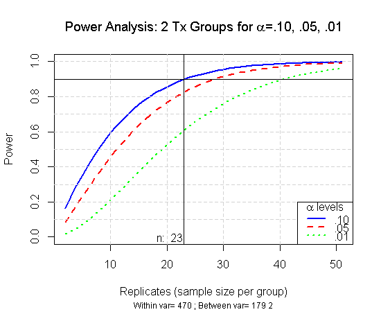
and power is calculated as power = 1 - \beta.

In order to calculate the probability of a Type II error a researcher needs to know a few pieces of information \mu, \sigma^2, n, and \alpha (probability of a Type I error). Normally, if a researcher already knows the population mean (\mu) and variance (\sigma^2) there is no need to take a sample to estimate them. However, we can set it up so we can look at a range of possible unknown population means and variances to see what the probability of a Type II error is for those values.

The following code shows a basic calculation and the density plot of a Type II error.

P\left(X>38| \mu,\sigma^2 \right)=P\left(Z>\frac{38-50}{10}\right)=P\left(Z>-1.2\right)=.8849303

my.means = c(38,50);
my.sd = c(10,10);

X = seq(my.means[1]-my.sd[1]*5,my.means[1]+my.sd[1]*5, length=100);
dX = dnorm(X, mean=my.means[1], sd=my.sd[1]); #True distribution
dX = dX/max(dX);

X.2 = seq(my.means[2]-my.sd[2]*5,my.means[2]+my.sd[2]*5, length=100);
dX.2 = dnorm(X.2, mean=my.means[2], sd=my.sd[2]); #Sampled distribution
dX.2 = dX.2/max(dX.2);

plot(X, dX, type="l", lty=1, lwd=2, xlab="x value",
ylab="Density", main="Comparison of Type II error probability",
xlim=c(min(X,X.2),max(X,X.2)))
lines(X.2,dX.2, lty=2)
abline(v=my.means, lty=c(1,2));
legend("topleft", c("Sample","Type II Error"), lty=c(2,1), col=c("black","black"), lwd=2, title=expression(paste("Type II Error")))

x = (my.means[1]-my.means[2])/my.sd[2];
1-pnorm(x);

[1] 0.8849303


However, there is a more direct way to determine necessary power and the Type II error calculation using R by setting up a range of sample sizes. Often the mean and variance for power analysis are established through a pilot study or other preliminary research on the population of interest.

R has several convenient functions to calculate power for many different types of tests and designs.  For this example power.anova.test will be used for demonstration purposes.  However, power.t.test could have been used as well.

For each of these functions there are varying values that need to be supplied however they generally involve effect size (difference in group means), sample size, alpha level, measure of variability and power.  In this example the within variability is estimated by using the MSE from the ANOVA table and the between variability is estimated from the variance of group means.  Otherwise, three different alpha levels are measured over a range of 50 possible n’s.


set.seed(1234);
x = matrix(NA,nrow=200,ncol=2);
x[,1]= rbind(rep(1,100),rep(2,100))
x[,2]= rbind(rnorm(100,23,20),rnorm(100,7,20));
x=data.frame(x); names(x) = c("group","value");
groupmeans = as.matrix(by(x$value,x$group,mean));
x.aov = summary(aov(x$value ~ as.factor(x$group)))

nlen = 50
withinvar = 470; ##From MSE in ANOVA
raw.pwr = matrix(NA, nrow=nlen, ncol=5)
for(i in 1:nlen){
pwr.i10 = power.anova.test(groups=length(groupmeans), n=1+i,
between.var=var(groupmeans), within.var=withinvar, sig.level=.10)
pwr.i05 = power.anova.test(groups=length(groupmeans), n=1+i,
between.var=var(groupmeans), within.var=withinvar, sig.level=.05)
pwr.i01 = power.anova.test(groups=length(groupmeans), n=1+i,
between.var=var(groupmeans), within.var=withinvar, sig.level=.01)
power10 = pwr.i10$power
power05 = pwr.i05$power
power01 = pwr.i01$power
raw.pwr[i,1] = power10
raw.pwr[i,2] = power05
raw.pwr[i,3] = power01
raw.pwr[i,5] = 1+i
}

plot(raw.pwr[,5], raw.pwr[,1], type="n", ylim=c(0,1),
ylab="Power",xlab="Replicates (sample size per group)",
main=expression(paste("Power Analysis: 2 Tx Groups for ", alpha, "=.10, .05, .01"))
, sub=paste("Within var=",withinvar,"; Between var=", round(var(groupmeans)),2), cex.sub=.75
)
lines(raw.pwr[,5], raw.pwr[,1], type="l", lty=1, lwd=2, col="blue")
lines(raw.pwr[,5], raw.pwr[,2], type="l", lty=2, lwd=2, col="red")
lines(raw.pwr[,5], raw.pwr[,3], type="l", lty=3, lwd=2, col="green")
abline(h=seq(.1:.9, by=.1), col="lightgrey", lty=2); abline(h=.9, col=1, lty=1);
abline(v=c(10,20,30,40), lty=2, col="lightgrey")
abline(v=raw.pwr[,5][round(raw.pwr[,1],2)==.90][1]); text(raw.pwr[,5][round(raw.pwr[,1],2)==.90][1]-2.5, 0, paste("n: ",raw.pwr[,5][round(raw.pwr[,1],2)==.90][1]));
legend("bottomright", c(".10",".05",".01"), lty=c(1,2,3), col=c("blue","red","green"), lwd=2, title=expression(paste(alpha, " levels")))

Power analysis over a range of n's

This graph shows what the power will be at a variety of sample sizes. In this example to obtain a power of 0.90 (\alpha=0.10) a sample of size 23 (per group) is needed.  So that will be a total of 46 observations.  It’s then up to the researcher to determine the appropriate sample size based on needed power, desired effect size, \alpha level, and cost.

There is no real fixed standard for power. However, 0.8 and 0.9 are often used. This means that the probability of a Type II error is 0.2 and 0.1, respectively. But it really comes down to whether the researcher is willing to accept a Type I error or a Type II error. For example, it’s probably better to erroneously have a healthy patient return for a follow-up test than it is to tell a sick patient they’re healthy.


Earthquakes Over the Past 7 Days

This is a brief example using the maps in R and to highlight a source of data.  This is real-time data and it comes from the U.S. Geological Survey.  This shows the location of earthquakes with magnitude of at least 1.0 in the lower 48 states.

library(maps)
library(maptools)
library(rgdal)

eq = read.table(file=”http://earthquake.usgs.gov/earthquakes/catalogs/eqs7day-M1.txt”, fill=TRUE, sep=”,”, header=T)
plot.new()
my.map <- map("state", interior = FALSE, plot=F) x.lim <- my.map$range[1:2]; x.lim[1] <- x.lim[1]-1; x.lim[2] <- x.lim[2]+1; y.lim <- my.map$range[3:4]; y.lim[1] <- y.lim[1]-1; y.lim[2] <- y.lim[2]+1; map("state", interior = FALSE, xlim=x.lim, ylim=y.lim) map("state", boundary = FALSE, col="gray", add = TRUE) title("Magnitude 1+ Earthquakes Over the Past 7 Days") eq$mag.size <- NULL eq$mag.size[eq$Magnitude>=1 & eq$Magnitude<2] <- .75 eq$mag.size[eq$Magnitude>=2 & eq$Magnitude<3] <- 1.0 eq$mag.size[eq$Magnitude>=3 & eq$Magnitude<4] <- 1.5 eq$mag.size[eq$Magnitude>=4] <- 2.0 eq$mag.col <- NULL eq$mag.col[eq$Magnitude>=1 & eq$Magnitude<2] <- 'blue' eq$mag.col[eq$Magnitude>=2 & eq$Magnitude<3] <- 'green' eq$mag.col[eq$Magnitude>=3 & eq$Magnitude<4] <- 'orange' eq$mag.col[eq$Magnitude>=4] <- 'red' points(x=eq$Lon,y=eq$Lat,pch=16,cex=eq$mag.size, col=eq$mag.col) eq$magnitude.text <- eq$Magnitude eq$magnitude.text[eq$Magnitude<4] <- NA text(x=eq$Lon,y=eq$Lat,col='black',labels=eq$magnitude.text,adj=c(2.5),cex=0.5) legend('bottomright',c('M 1-2','M 2-3','M 3-4','M4+'), ncol=2, pch=16, col=c('blue','green','orange','red')) box() [/sourcecode]

Hurricane Sandy Land Wind Speed and Kriging

NJ Hurricane Sandy Landfall Data

These data come from the National Climatic Data Center (NCDC).  Using the above link will download all of the data collected by the NCDC on the day of Hurricane Sandy.  The data can also be obtained directly from the source at http://cdo.ncdc.noaa.gov/qclcd/QCLCD.

The purpose of this post is not a discussion on kriging or any of its properties. The purpose is to simply provide a simple R example on kriging and how it can be applied on real data.   This R code uses Hurricane Sandy as an example and predicts the wind speed across the state of New Jersey using the measurement stations that the NCDC uses. It is easy to see how this technique can be applied to other data.


wd <- "C:\\nj hurricane data" setwd(wd) my.files <- dir(wd, pattern = ".txt", full.names = TRUE, ignore.case = TRUE) krig <- matrix(NA, nrow=length(my.files), ncol=3) for(i in 1:length(my.files)){ raw <- read.csv(my.files[i], skip=6, header=T) raw <- subset(raw, raw$Date=="20121029") latlongraw <- read.csv(my.files[i], skip=3, header=F, sep="") latlongrows <- head(latlongraw,2)[,2] latlong <- as.numeric(levels(latlongrows)[latlongrows]) raw$WindSpeed[raw$WindSpeed=="M"] <- NA if(is.factor(raw$WindSpeed)){ raw$WindSpeed <- as.numeric(levels(raw$WindSpeed)[raw$WindSpeed]) } krig[i,1] <- latlong[1] krig[i,2] <- latlong[2] krig[i,3] <- max(raw$WindSpeed, na.rm=T) } lat <- krig[,1] long <- krig[,2] s<-cbind(long,lat) PM <- krig[,3] sandy$coords <- s sandy$data <- PM ml <- likfit(sandy, fix.nugget=F, cov.model="exponential", ini = c(10, 5), nugget=4) ml summary(ml) grid <- map("state","new jersey", plot=FALSE) grid.plot <- cbind( c(min(grid$x, na.rm=TRUE),max(grid$x, na.rm=TRUE)), c(min(grid$y, na.rm=TRUE),max(grid$y, na.rm=TRUE)) ) sp1<-seq(grid.plot[1,1]-.25,grid.plot[2,1]+.25,length=100) sp2<-seq(grid.plot[1,2]-.25,grid.plot[2,2]+.25,length=100) sp<-expand.grid(sp1,sp2) inLoc<-map.where("state",x=sp[,1],y=sp[,2]) inLoc[is.na(inLoc)]<-"NA" inLoc<-inLoc=="new jersey" #Perform ordinary Kriging (value of cov.pars and nugget are copied from mle output): pred<-krige.conv(data=PM,coords=s,locations=sp, krige=krige.control(type.krige="ok",cov.model="exponential", cov.pars=c(100,3), nugget=5)) pred$predict[!inLoc]<-NA pred$krige.var[!inLoc]<-NA #Plot the predicted values: image.plot(sp1,sp2,matrix(pred$predict,100,100),zlim=range(PM), main="Sandy Maximum Wind Speed in MPH", xlab="Longitude",ylab="Latitude") map("county",add=T) points(s, pch=16) [/sourcecode]

What Time Is It?

A common scenario that I run into is time and how to deal with it. I often will do a  variety of summaries and analysis that need to be measured at different points in time. Whether I want to graph the data or review the results I need to be able to perform measurements relative to time and interpret the time output in human readable form. R has several functions to handle those time related scenario.

For starters one thing needs to be acknowledged. On Unix based system the beginning of time is January 1, 1970. At that moment exactly zero (0) seconds have passed and it is known as Unix epoch. Anything before that is negative and anything after that time is positive. This measure of time is defined in seconds.

This piece of code shows the Unix epoch and how it compares to the current time.  In this example the origin is zero (0) but as one can see it can easily be changed to calculate the length of time that has past since any given time.

##Local Time in EDT (GMT-5). If local time IS GMT then the date would be January 1, 1970
iso <- ISOdatetime(1969,12,31,19,0,0) # (YYYY,MM,DD,HH,MM,SS) origin <- as.double(iso) t <- Sys.time() curr.time <- as.double(t) curr.time - origin [/sourcecode]   The following bit of code simulates a cumulative process where each consecutive process follows a Poisson distribution  and [latex]\lambda[/latex] (lambda) is a random variable distributed uniformly.  This would be comparable to a process where election vote counts are being collected throughout Election Night. [sourcecode language="css"] set.seed(1234) time.series <- seq(Sys.time(), Sys.time()+4*60*60, by=60*5) #Add 4 hours to time series vals <- matrix(NA, ncol=3, nrow=length(time.series)) for(i in 1:length(time.series)){ if( is.numeric(vals[i-1,1]) & is.numeric(vals[i-1,2]) ){ vals[i,1] <- vals[i-1,1]+rpois(n=1, runif(1, 700,1000)) vals[i,2] <- vals[i-1,2]+rpois(n=1, runif(1, 850,1000)) } else { vals[i,1] <- runif(1, 700,1000) vals[i,2] <- runif(1, 850,1000) } } vals[,3] <- vals[,1]/(vals[,1]+vals[,2]) prop <- vals[,3]*100 prop2 <- (1-vals[,3])*100 plot(time.series,prop, type="o", cex=.6, lty=1, col="blue", pch=1, ylim=c(46,54) , ylab="Percent", xlab="Time of Computation" , main=paste("Example of Cumulative Process Using Time") , sub="Cumulative Proportional Process", cex.sub=.60 , xaxt = "n", yaxt = "n"); lines(time.series, prop2, type="o", cex=.6, lty=1, col="red", pch=4); xaxis.seq.half<- seq(strptime(c(min(time.series)), "%Y-%m-%d %H"), strptime(c(max(time.series)), "%Y-%m-%d %H")+3600, by=1800) xaxis.seq.hour <- seq(strptime(c(min(time.series)), "%Y-%m-%d %H"), strptime(c(max(time.series)), "%Y-%m-%d %H")+3600, by=3600) axis(1, at=(xaxis.seq.hour), tcl = -0.7, lty = 1, lwd = 0.8, labels=FALSE) axis(1, at=(xaxis.seq.half), tcl = -0.3, lty = 2, lwd = 0.5, labels=FALSE) axis(2, at=seq(46,54,by=1), labels=FALSE, tcl = -0.2, lty = 1, lwd = 0.5) axis(2, at=seq(46,54,by=1), labels=TRUE, tcl = -0.7, lty = 1) axis.POSIXct(1, as.POSIXlt(xaxis.seq.hour), at=as.POSIXlt(xaxis.seq.hour), format="%H:%M", tcl = 0.3, las=0, lty = 2, lwd = 0.5, cex.axis=.7, labels=TRUE) [/sourcecode]

One Big Number That’s Not Big Enough

32-bit systems pose an interesting problem because of some of its limitations. These systems are only capable of handling an integer that is  2^{63}-1 = 2147483647.   That is a fairly large number but it just not large enough.  That is particularly true if that number is a phone number (e.g. (214)748-3647).  As you can see there would be a large block of numbers that would cause problems.  In other words a phone number is not an integer and should not be cast as an integer, ever!  Normally on 32-bit systems if an integer exceeds that number it will either kindly return an error or it will send you back in time to the year 1901.  Neither one of those options are very good.  The solution: upgrade to a 64-bit system.  That will allow for a maximum integer of 9,223,372,036,854,775,807.  A 64-bit system will be good for another 292 million years.  The time solution is then solved.  However, it’s not out of the question that there could be a scenario when a researcher will exceed 9.2 quintillion.  This could be the case when dealing with large data mining and trying to analyze something like each grain of sand on a beach.  But I guess then it’s time to upgrade again to something bigger.

Note that when dealing with numbers and computers they normally begin at 0.  So at index 31 you have actually reach the 32nd position and therefore a 32-bit system.  Likewise, 2^{63}-1 = 9223372036854775807.

If you’re not certain then you can quickly find out what the maximum allowable integer by using any of the following lines of code.

In R you can identify the maximum integer:

.Machine$integer.max

In Perl you can identify dates that go back on time:

#!/usr/local/bin/perl

use POSIX;
$ENV{‘TZ’} = “GMT”;

for ($clock = 2147483641; $clock < 2147483651; $clock++) { print ctime($clock); } [/sourcecode] In PHP this is the same as the Perl script: [sourcecode language="css"]

Using R to Compare Hurricane Sandy and Hurricane Irene

Having just lived through two back to back hurricanes (Irene in 2011 and Sandy in 2012) that passed through the New York metro area I was curious how the paths of the hurricanes differed.  I worked up a quick graph in R using data from Unisys.  The data also includes wind speed and barometric pressure.

library(maps)
library(maptools)
library(rgdal)

sandy = read.table(file=”http://weather.unisys.com/hurricane/atlantic/2012/SANDY/track.dat”, skip=3,fill=TRUE)
irene = read.table(file=”http://weather.unisys.com/hurricane/atlantic/2011H/IRENE/track.dat”,skip=3,fill=TRUE)
colnames(sandy) = c(“Advisory”,”Latitude”,”Longitude”,”Time”,”WindSpeed”,”Pressure”,”Status”)
colnames(irene) = c(“Advisory”,”Latitude”,”Longitude”,”Time”,”WindSpeed”,”Pressure”,”Status”)

sandy$WindSpeedColor <- 'blue' sandy$WindSpeedColor[sandy$WindSpeed >= 75] <- 'red' irene$WindSpeedColor <- 'blue' irene$WindSpeedColor[sandy$WindSpeed >= 75] <- 'red' xlim <- c(-88,-65) ylim <- c(25,48) state.list <- c('new york','new jersey','virginia','massachusetts','connecticut','delaware','pennsylvania','maryland','north carolina','south carolina','georgia','florida', 'new hampshire','maine','district of columbia','west virginia','vermont') my.map <- map("state", region = state.list, interior = FALSE, xlim=xlim, ylim=ylim) map("state", region = state.list, boundary = FALSE, col="gray", add = TRUE,xlim=xlim) lines(x=sandy$Longitude,y=sandy$Latitude,col="black",cex=0.75) points(x=sandy$Longitude,y=sandy$Latitude,col=sandy$WindSpeedColor,pch=15,cex=0.9) text(x=sandy$Longitude,y=sandy$Latitude,col='dark green',labels=sandy$Pressure,adj=c(-0.9),cex=0.5) lines(x=irene$Longitude,y=irene$Latitude,col="black",cex=0.75) points(x=irene$Longitude,y=irene$Latitude,col=irene$WindSpeedColor,pch=15,cex=0.9) text(x=irene$Longitude,y=irene$Latitude,col='light green',labels=irene$Pressure,adj=c(-0.9),cex=0.5) title("Path of Hurricane Sandy (2012) and Hurricane Irene (2011)\nwith Wind Speed and Barometric Pressure") legend('topleft',c('Tropical Storm Wind Speeds','Hurricane Wind Speeds'),pch=15, col=c('blue','red')) box() [/sourcecode]  


Mapping Capabilities in R

From time-to-time creating a basic map of the United States or other parts of the world to complement some statistical analysis is useful to emphasize a point. The maps package in R provide a good way to produce these these maps.  These maps axes are based on latitude and longitude so overlaying other information on these maps is quite simple.  Furthermore, it makes a nice addition to geo-spatial analysis.

This is a simple introductory example that is designed to show a couple of different examples.  First, it shows the USA lower 48 states database and how it can be used to create the state boundaries.  Second, the world database is used to add Alaska and Hawaii.  A nice feature is that the colors for each of the state boundaries can be easily changed to group states.   This (non-optimized) code shows a basic example on how to use the maps package to show the Election Day poll closing times for all 50 states and the District of Columbia.

library(maps)
m <- map("state", interior = FALSE, plot=FALSE) m$my.colors <- 0 m$my.colors[m$names %in% c("virginia:main","georgia","vermont","kentucky","indiana","south carolina")] <- 2 m$my.colors[m$names %in% c("west virginia","north carolina:main","ohio")] <- 3 m$my.colors[m$names %in% c("tennessee","rhode island","oklahoma","new jersey","mississippi","massachusetts:main","illinois","maryland","maine","missouri","new hampshire","new jersey","pennsylvania","florida","connecticut","delaware","district of columbia","alabama")] <- 4 m$my.colors[m$names %in% c("arkansas")] <- 5 m$my.colors[m$names %in% c("arizona","colorado","kansas","louisiana","minnesota","michigan:north","michigan:south","nebraska","new york:main","new york:manhattan","new york:staten island","new york:long island","new mexico","north dakota","south dakota","texas","wyoming","wisconsin")] <- 6 m$my.colors[m$names %in% c("iowa","montana","nevada","utah")] <- 7 m$my.colors[m$names %in% c("california","idaho","oregon","washington:main")] <- 8 m.world <- map("world", c("USA","hawaii"), xlim=c(-180,-65), ylim=c(19,72),interior = FALSE) title("Election Day Poll Closing Times") map("state", boundary = FALSE, col="grey", add = TRUE, fill=FALSE) map("state", boundary = TRUE, col=m$my.colors, add = TRUE, fill=TRUE ) map("world", c("hawaii"), boundary = TRUE, col=8, add = TRUE, fill=TRUE ) map("world", c("USA:Alaska"), boundary = TRUE, col='orange', add = TRUE, fill=TRUE ) legend("topright", c('7:00pm','7:30pm','8:00pm','8:30pm','9:00pm','10:00pm','11:00pm','1:00am'), pch=15, col=c(2,3,4,5,6,7,8,'orange'), title="Poll Closing Time (EST)", ncol=2, cex=1.2) [/sourcecode] Because the maps are based on longitude and latitude this package can be extended beyond just county, state and country boundaries and can be used on techniques like kriging and co-kriging to develop model-based maps.

Text Mining

When it comes down to it R does a really good job handling structured data like matrices and data frames. However, its ability to work with unstructured data is still a work in progress. It can and it does handle text mining but the documentation is incomplete and the capabilities still don’t compare to other programs such as MALLET or Mahout.

Though the formal documentation is still lacking. Though this is not an example on real data it does provide the basic tools on text mining and, in particular, latent dirichlet allocation.

There are three R libraries that are useful for text mining: tm, RTextTools, and topicmodels. The tm library is the core of text mining capabilities in R.

Unstructured text files can come in many different formats. I often find that I must get my own data and consequently the data generally originates as plain text (.txt) files. However, those who want to analyze Twitter feeds can user the twitteR library which is useful for analyzing social media topics in real time. This example will incorporate the CNN twitter feed.

In order for R to interpret and analyze these text files they must ultimately be converted into a document term matrix. But first a corpus must be created. A corpus is simply a collection of documents where each document its a topic.

When reading text documents directly from local file the following R code can be used.

Data Preparation using Local Text Files


#These files can be just raw text. For example it could be simply copied and pasted from a Web site.
dir = "C:\\Documents and Settings\\clints\\My Documents\\LDA-S";
filenames = list.files(path=dir,pattern="\\.txt");
setwd(dir);

docs = NULL;
titles = NULL;

for (filename in filenames){
#here I specify a file that contains all the titles of the documents
if(filename=="titles.txt"){
titles = paste(readLines(file(filename)));
} else {
docs = c(docs,list( paste(readLines(file(filename)), collapse="\n") ));
}
}

To pull the text from a Twitter Feed rather than text files then the following lines of code can be used.

Data Preparation using Twitter


library(tm);
library(RTextTools);
library(topicmodels);
library(twitteR);

twitter_feed <- searchTwitter('@cnn', n=150);

### Optional twitter feed retrieval
##twitter_feed <- userTimeline("rdatamining", n=150);
###

df <- do.call("rbind", lapply(twitter_feed, as.data.frame));
myCorpus <- Corpus(VectorSource(df$text));

k = length(docs3);
myCorpus = Corpus(VectorSource(docs));
myCorpus = tm_map(myCorpus, tolower);
myCorpus = tm_map(myCorpus, removePunctuation);
myCorpus = tm_map(myCorpus, removeNumbers);
myStopwords = c(stopwords('english'), "available", "via");
idx = which(myStopwords == "r");
myStopwords = myStopwords&#91;-idx&#93;;
myCorpus = tm_map(myCorpus, removeWords, myStopwords);

dictCorpus = myCorpus;

myCorpus = tm_map(myCorpus, stemDocument);

myCorpus = tm_map(myCorpus, stemCompletion, dictionary=dictCorpus);

myDtm = DocumentTermMatrix(myCorpus, control = list(minWordLength = 3));

findFreqTerms(myDtm, lowfreq=50);
#find the probability a word is associated
findAssocs(myDtm, 'find_a_word', 0.5);

&#91;/sourcecode&#93;

<strong>Word Cloud</strong>


library(wordcloud);
m = as.matrix(myDtm);
v = sort(colSums(m), decreasing=TRUE);
myNames = names(v);
k = which(names(v)=="miners");
myNames[k] = "mining";
d = data.frame(word=myNames, freq=v);
wordcloud(d$word, colors=c(3,4), random.color=FALSE, d$freq, min.freq=20);

Latent Dirichlet Allocation


k = 2;
SEED = 1234;
my_TM =
list(VEM = LDA(myDtm, k = k, control = list(seed = SEED)),
VEM_fixed = LDA(myDtm, k = k,
control = list(estimate.alpha = FALSE, seed = SEED)),
Gibbs = LDA(myDtm, k = k, method = "Gibbs",
control = list(seed = SEED, burnin = 1000,
thin = 100, iter = 1000)),
CTM = CTM(myDtm, k = k,
control = list(seed = SEED,
var = list(tol = 10^-4), em = list(tol = 10^-3))));

Topic = topics(my_TM[["VEM"]], 1);

#top 5 terms for each topic in LDA
Terms = terms(my_TM[["VEM"]], 5);
Terms;

(my_topics =
topics(my_TM[["VEM"]]));

most_frequent = which.max(tabulate(my_topics));

terms(my_TM[["VEM"]], 10)[, most_frequent];

Here, a model is fit setting the number of unobserved latent topics equal to two (k=2). We can then identify the most frequently occurring topics and then identify the top five terms used for the topic. In this example these are the top five terms when setting the number of groups equal to two.

Topic 1 Topic 2
“amp” “cnn”
“cnn” “tweet”
“jobs” “abc”
“romney” “bainport”
“sensata” “cbs”