Power Analysis and the Probability of Errors

Power analysis is a very useful tool to estimate the statistical power from a study. It effectively allows a researcher to determine the needed sample size in order to obtained the required statistical power. Clients often ask (and rightfully so) what the sample size should be for a proposed project. Sample sizes end up being a delicate balance between the amount of acceptable error, detectable effect size, power, and financial cost. A lot of factors go into this decision. This example will discuss one approach.

In more specific terms power is the probability that a statistical test will reject the null hypothesis when the null hypothesis is truly false. What this means is that when power increases the probability of making a Type II error decreases. The probability of a Type II error is denoted by and power is calculated as .

In order to calculate the probability of a Type II error a researcher needs to know a few pieces of information , , , and (probability of a Type I error). Normally, if a researcher already knows the population mean () and variance () there is no need to take a sample to estimate them. However, we can set it up so we can look at a range of possible unknown population means and variances to see what the probability of a Type II error is for those values.

The following code shows a basic calculation and the density plot of a Type II error.

my.means = c(38,50);
my.sd = c(10,10);

X = seq(my.means[1]-my.sd[1]*5,my.means[1]+my.sd[1]*5, length=100);
dX = dnorm(X, mean=my.means[1], sd=my.sd[1]); #True distribution
dX = dX/max(dX);

X.2 = seq(my.means[2]-my.sd[2]*5,my.means[2]+my.sd[2]*5, length=100);
dX.2 = dnorm(X.2, mean=my.means[2], sd=my.sd[2]); #Sampled distribution
dX.2 = dX.2/max(dX.2);

plot(X, dX, type="l", lty=1, lwd=2, xlab="x value",
ylab="Density", main="Comparison of Type II error probability",
xlim=c(min(X,X.2),max(X,X.2)))
lines(X.2,dX.2, lty=2)
abline(v=my.means, lty=c(1,2));
legend("topleft", c("Sample","Type II Error"), lty=c(2,1), col=c("black","black"), lwd=2, title=expression(paste("Type II Error")))

x = (my.means[1]-my.means[2])/my.sd[2];
1-pnorm(x);

[1] 0.8849303

 

 

However, there is a more direct way to determine necessary power and the Type II error calculation using R by setting up a range of sample sizes. Often the mean and variance for power analysis are established through a pilot study or other preliminary research on the population of interest.

R has several convenient functions to calculate power for many different types of tests and designs.  For this example power.anova.test will be used for demonstration purposes.  However, power.t.test could have been used as well.

For each of these functions there are varying values that need to be supplied however they generally involve effect size (difference in group means), sample size, alpha level, measure of variability and power.  In this example the within variability is estimated by using the MSE from the ANOVA table and the between variability is estimated from the variance of group means.  Otherwise, three different alpha levels are measured over a range of 50 possible n’s.

set.seed(1234);
x = matrix(NA,nrow=200,ncol=2);
x[,1]= rbind(rep(1,100),rep(2,100))
x[,2]= rbind(rnorm(100,23,20),rnorm(100,7,20));
x=data.frame(x); names(x) = c("group","value");
groupmeans = as.matrix(by(x$value,x$group,mean));
x.aov = summary(aov(x$value ~ as.factor(x$group)))

nlen = 50
withinvar = 470; ##From MSE in ANOVA
raw.pwr = matrix(NA, nrow=nlen, ncol=5)
for(i in 1:nlen){
pwr.i10 = power.anova.test(groups=length(groupmeans), n=1+i,
between.var=var(groupmeans), within.var=withinvar, sig.level=.10)
pwr.i05 = power.anova.test(groups=length(groupmeans), n=1+i,
between.var=var(groupmeans), within.var=withinvar, sig.level=.05)
pwr.i01 = power.anova.test(groups=length(groupmeans), n=1+i,
between.var=var(groupmeans), within.var=withinvar, sig.level=.01)
power10 = pwr.i10$power
power05 = pwr.i05$power
power01 = pwr.i01$power
raw.pwr[i,1] = power10
raw.pwr[i,2] = power05
raw.pwr[i,3] = power01
raw.pwr[i,5] = 1+i
}

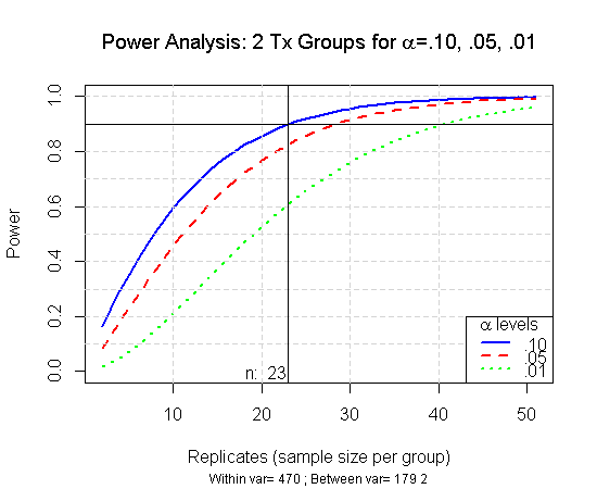
plot(raw.pwr[,5], raw.pwr[,1], type="n", ylim=c(0,1),
ylab="Power",xlab="Replicates (sample size per group)",
main=expression(paste("Power Analysis: 2 Tx Groups for ", alpha, "=.10, .05, .01"))
, sub=paste("Within var=",withinvar,"; Between var=", round(var(groupmeans)),2), cex.sub=.75
)
lines(raw.pwr[,5], raw.pwr[,1], type="l", lty=1, lwd=2, col="blue")
lines(raw.pwr[,5], raw.pwr[,2], type="l", lty=2, lwd=2, col="red")
lines(raw.pwr[,5], raw.pwr[,3], type="l", lty=3, lwd=2, col="green")
abline(h=seq(.1:.9, by=.1), col="lightgrey", lty=2); abline(h=.9, col=1, lty=1);
abline(v=c(10,20,30,40), lty=2, col="lightgrey")
abline(v=raw.pwr[,5][round(raw.pwr[,1],2)==.90][1]); text(raw.pwr[,5][round(raw.pwr[,1],2)==.90][1]-2.5, 0, paste("n: ",raw.pwr[,5][round(raw.pwr[,1],2)==.90][1]));
legend("bottomright", c(".10",".05",".01"), lty=c(1,2,3), col=c("blue","red","green"), lwd=2, title=expression(paste(alpha, " levels")))

This graph shows what the power will be at a variety of sample sizes. In this example to obtain a power of 0.90 () a sample of size 23 (per group) is needed.  So that will be a total of 46 observations.  It’s then up to the researcher to determine the appropriate sample size based on needed power, desired effect size, level, and cost.

There is no real fixed standard for power. However, 0.8 and 0.9 are often used. This means that the probability of a Type II error is 0.2 and 0.1, respectively. But it really comes down to whether the researcher is willing to accept a Type I error or a Type II error. For example, it’s probably better to erroneously have a healthy patient return for a follow-up test than it is to tell a sick patient they’re healthy.